Open Physics Letters Logo
AnalysesArticlesCoursesProblemsGreat PhysicistsBooks in Physics History
TRTRENEN
Open Physics Letters

Open Physics Letters provides free access to academic analyses, historical breakthroughs, and educational resources in physics — from high school to postgraduate level.

TR

Academic Content

  • auto_storiesArticles
  • psychologyAnalyses
  • personGreat Physicists
  • menu_bookBooks in Physics History

Education

  • schoolCourses
  • calculateProblem Solutions

Institute

  • About Us
  • Contact
  • Contribute
  • Privacy Policy
  • Terms of Service

© 2026 Open Physics Letters Academic Press. All rights reserved.

TRTR|ENEN
Courseschevron_rightClassical Mechanicschevron_rightClassical Mechanics: A Textbook-Based Course Based on Classical Dynamics of Particles and Systemschevron_rightVectors, Matrice and Vector Calculus-Mathematical Foundationschevron_rightProperties of Rotation Matrices

1.4 Properties of Rotation Matrices

summarize

Summary

This section introduces rotation matrices using direction cosines. It explains how rotations are represented using cosine relationships between coordinate axes and shows that rotation matrices are orthogonal matrices whose inverse equals their transpose. The section also explains coordinate transformations for rotated coordinate systems.

target

Learning Objectives

  • 1.Understand direction cosines and their geometric meaning
  • 2.Understand how rotation matrices are constructed
  • 3.Understand orthogonality conditions of rotation matrices
  • 4.Apply coordinate transformation formulas
library_books

Related Topic in Source

menu_bookClassical Dynamics of Particles and Systems
subdirectory_arrow_rightMatrices, Vectors, and Vector Calculus
arrow_rightProperties of Rotation Matrices

Direction Cosines

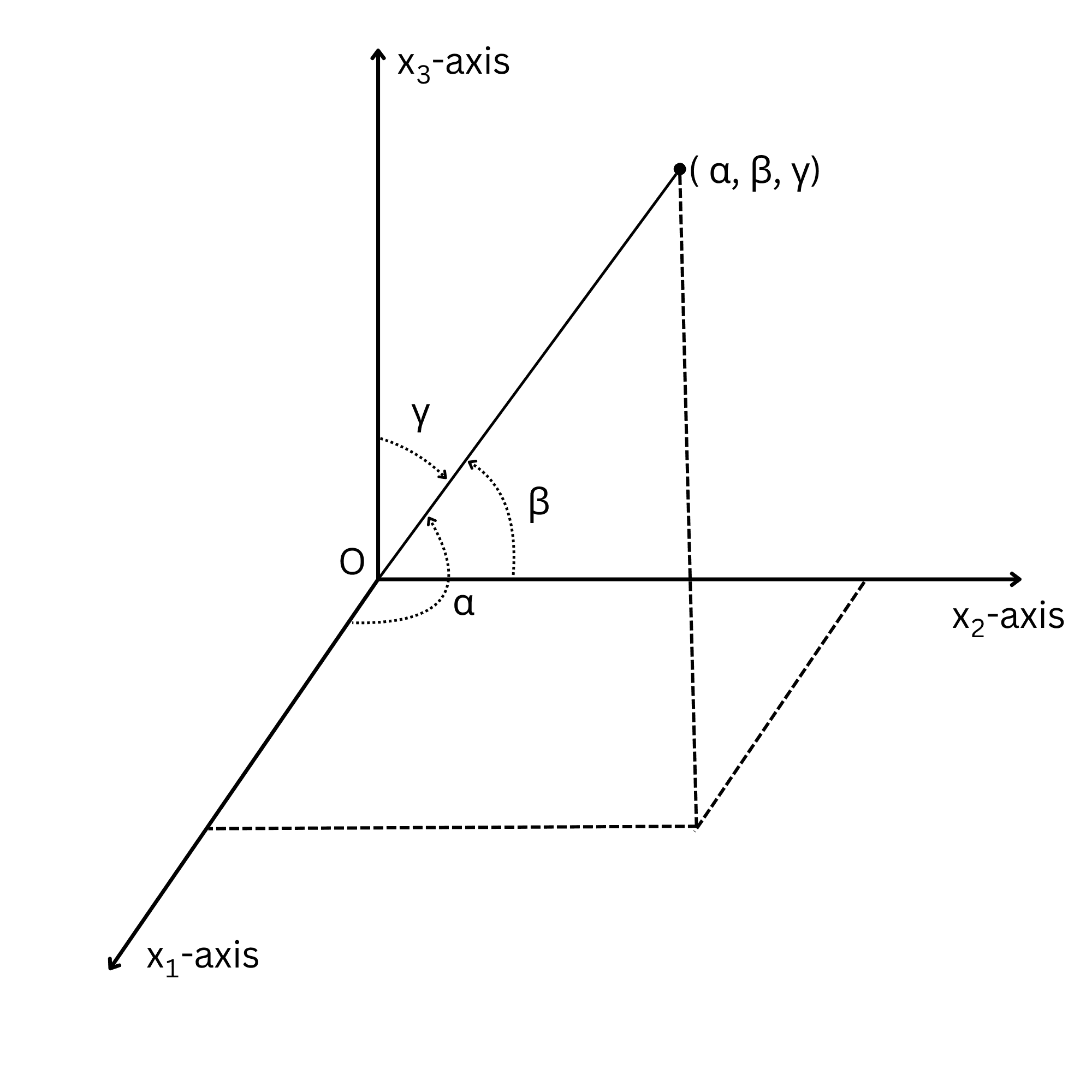
Consider a line passing through the origin in three-dimensional space. The line forms angles with the coordinate axes x1x_1x1​, x2x_2x2​, and x3x_3x3​. Let these angles be α\alphaα, β\betaβ, and γ\gammaγ. (See Figure 1) The cosines of these angles are called direction cosines and describe the orientation of the line.

cos⁡2α+cos⁡2β+cos⁡2γ=1\cos^2 \alpha + \cos^2 \beta + \cos^2 \gamma = 1cos2α+cos2β+cos2γ=1

The squares of the direction cosines always sum to one because they represent the components of a unit direction vector.

Figure 1
Figure 1

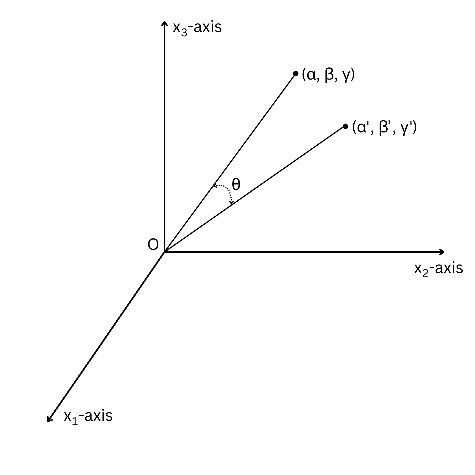
If two lines are given by direction cosines (cos⁡α,cos⁡β,cos⁡γ)(\cos \alpha, \cos \beta, \cos \gamma)(cosα,cosβ,cosγ) and (cos⁡α′,cos⁡β′,cos⁡γ′)(\cos \alpha', \cos \beta', \cos \gamma')(cosα′,cosβ′,cosγ′), then the cosine of the angle between the lines is equal to the dot product of the direction cosine vectors. (See Figure 2)

cos⁡θ=cos⁡αcos⁡α′+cos⁡βcos⁡β′+cos⁡γcos⁡γ′\cos \theta = \cos \alpha \cos \alpha' + \cos \beta \cos \beta' + \cos \gamma \cos \gamma'cosθ=cosαcosα′+cosβcosβ′+cosγcosγ′

The angle between two lines is computed using the dot product of their unit direction vectors.

Figure 2
Figure 2

Rotation Matrix Definition

A rotation of a coordinate system can be described by the cosines of the angles between the original axes (x1,x2,x3)(x_1,x_2,x_3)(x1​,x2​,x3​) and the rotated axes (x1′,x2′,x3′)(x'_1,x'_2,x'_3)(x1′​,x2′​,x3′​). These cosines are written as λij\lambda_{ij}λij​ and form the rotation matrix.

λij=cos⁡(xi′,xj)\lambda_{ij} = \cos(x'_i , x_j)λij​=cos(xi′​,xj​)

Each element of the rotation matrix represents the cosine of the angle between a rotated axis and an original axis.

Although the rotation matrix contains nine elements, only three are independent because the coordinate axes must remain perpendicular and have unit length.

Orthogonality Conditions

Since the rotated coordinate axes remain perpendicular to each other, the direction cosines must satisfy orthogonality conditions. These conditions ensure that different axes remain perpendicular after rotation.

∑jλijλkj=0(i≠k)\sum_j \lambda_{ij} \lambda_{kj} = 0 \quad (i \neq k)j∑​λij​λkj​=0(i=k)

Different rows of the rotation matrix are orthogonal

∑jλijλij=1\sum_j \lambda_{ij} \lambda_{ij} = 1j∑​λij​λij​=1

Each axis has unit length after rotation.

∑jλijλkj=δik\sum_j \lambda_{ij} \lambda_{kj} = \delta_{ik}j∑​λij​λkj​=δik​

The rows of the rotation matrix form an orthonormal set of vectors

δik=0  (i≠k),δik=1  (i=k)\delta_{ik} = 0 \; (i \neq k), \quad \delta_{ik} = 1 \; (i = k)δik​=0(i=k),δik​=1(i=k)

The Kronecker delta distinguishes equal and unequal indices

Column Orthogonality

The same reasoning can be applied by expressing the original axes in terms of the rotated axes. This produces a second orthogonality condition showing that the columns of the rotation matrix are also orthonormal.

∑iλijλik=δjk\sum_i \lambda_{ij} \lambda_{ik} = \delta_{jk}i∑​λij​λik​=δjk​

The columns of a rotation matrix are orthonormal vectors.

λ−1=λT\lambda^{-1} = \lambda^Tλ−1=λT

The inverse of a rotation matrix is equal to its transpose.

Rotation Interpretation

A rotation transformation can be interpreted in two equivalent ways. Either the coordinate axes rotate while the point remains fixed, or the coordinate axes remain fixed while the point rotates. Both interpretations produce the same transformation matrix.

Coordinate Transformation

Consider a point with coordinates (x1,x2)(x_1,x_2)(x1​,x2​) in the original coordinate system. After a rotation through an angle theta\\thetatheta, the coordinates in the rotated system become:

x1′=x1cos⁡θ+x2sin⁡θx^\prime_1 = x_1 \cos \theta + x_2 \sin \thetax1′​=x1​cosθ+x2​sinθ

First coordinate after rotation.

x2′=−x1sin⁡θ+x2cos⁡θx^\prime_2 = -x_1 \sin \theta + x_2 \cos \thetax2′​=−x1​sinθ+x2​cosθ

Second coordinate after rotation.

(x1′x2′)=(cos⁡θsin⁡θ−sin⁡θcos⁡θ)(x1x2)\begin{pmatrix} x^\prime_1 \\ x^\prime_2 \end{pmatrix} = \begin{pmatrix} \cos\theta & \sin \theta \\ -\sin \theta & \cos \theta \end{pmatrix} \begin{pmatrix} x_1 \\ x_2 \end{pmatrix}(x1′​x2′​​)=(cosθ−sinθ​sinθcosθ​)(x1​x2​​)

Matrix representation of a two-dimensional rotation.

menu_bookGo to Chapter
arrow_back
Previous Section

Coordinate Transformations