1.3 Coordinate Transformations

Imagine you know the coordinates of a point $P$ as $(x_1,x_2,x_3)$ in a given Cartesian coordinate system. Now suppose someone else is using a different set of axes — one that has been rotated relative to yours. How would you express the same point $P$ in their system $(x_1^{\prime },x_2^{\prime },x_3^{\prime })$?

This is the central question of coordinate transformations. They provide a systematic way to convert coordinates from one reference frame to another when the two frames differ by a rotation.

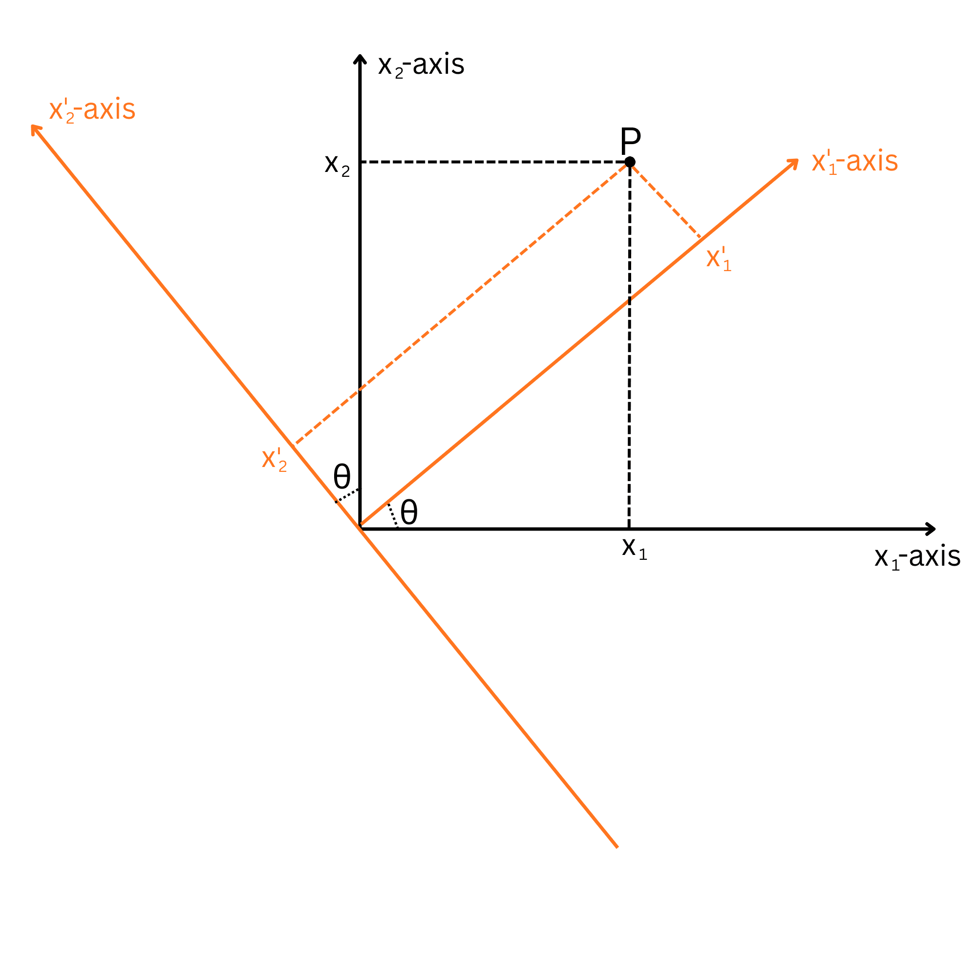
Let's start with two dimensions. Suppose the new coordinate axes $(x_1^{\prime },x_2^{\prime })$ are obtained by rotating the original axes $(x_1,x_2)$ by an angle $\theta$. (see Figure 1)

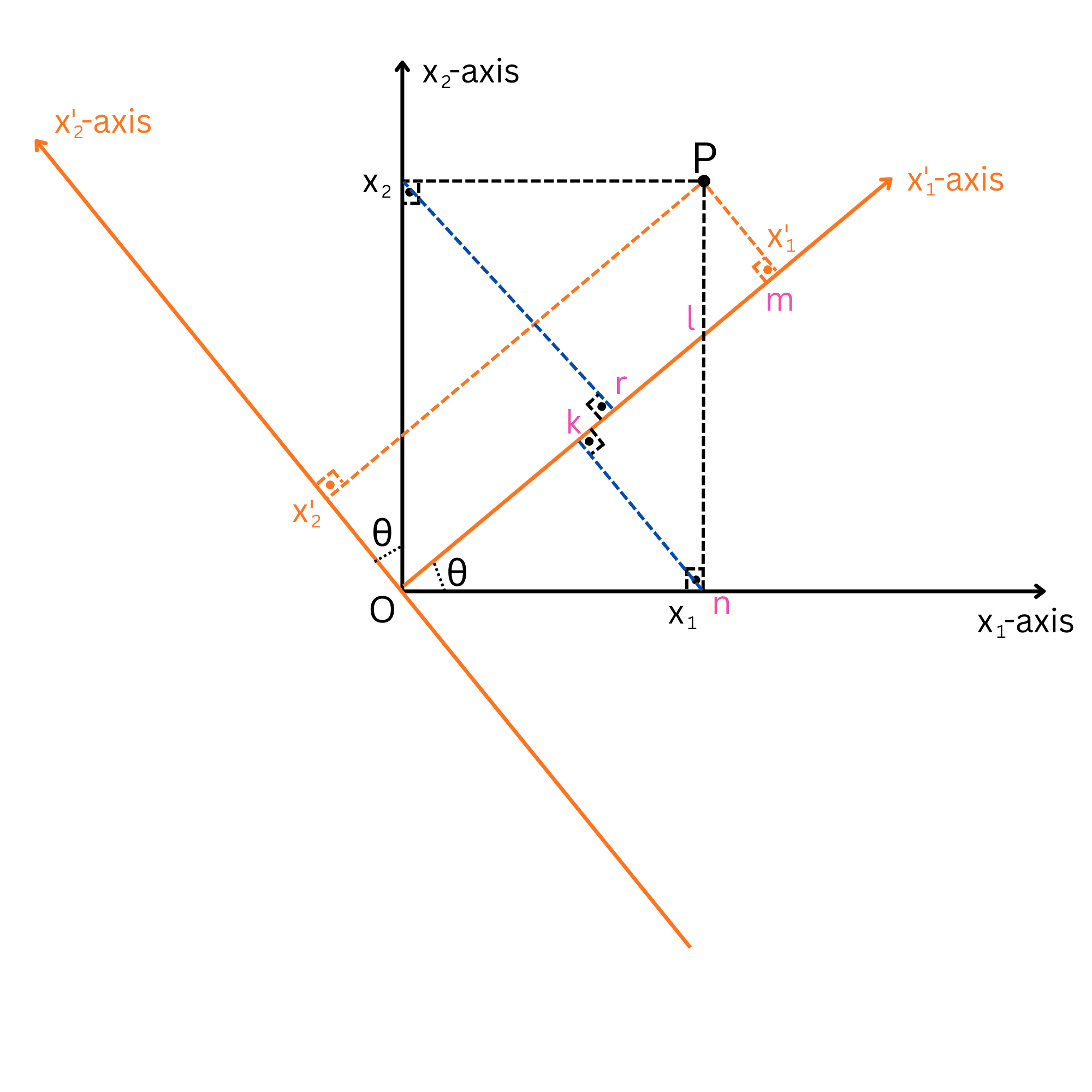
To find the new coordinate $x_1^{\prime }$, we project the original coordinates onto the new $x_1^{\prime }$-axis. (See Figure 2, blue lines)

In Figure 2, label the points as $k$, $l$, $m$, $n$, and $r$. Then, write the projection of $x_1$ onto $x_1^{\prime }$ and the projection of $x_2$ onto $x_1^{\prime }$:
${\mathrm{proj}}_{x_1^{\prime }}{x}_1=Ok‾=x_1\cos \theta$
${\mathrm{proj}}_{x_1^{\prime }}{x}_2=Or‾=x_2\sin \theta$

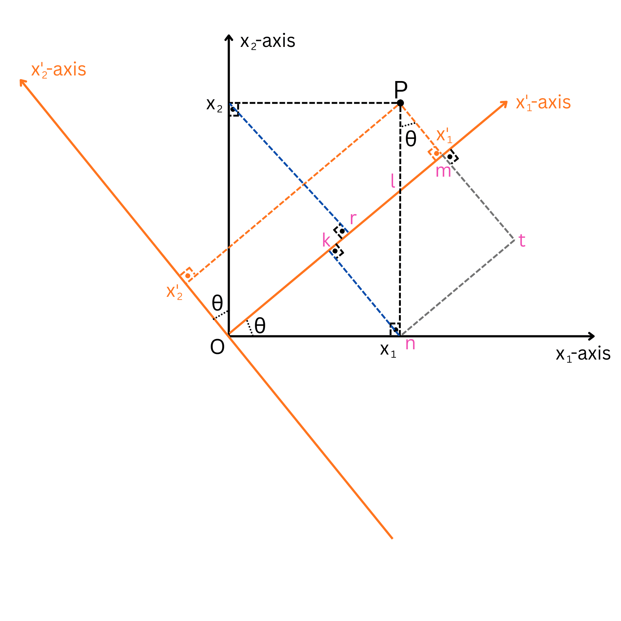
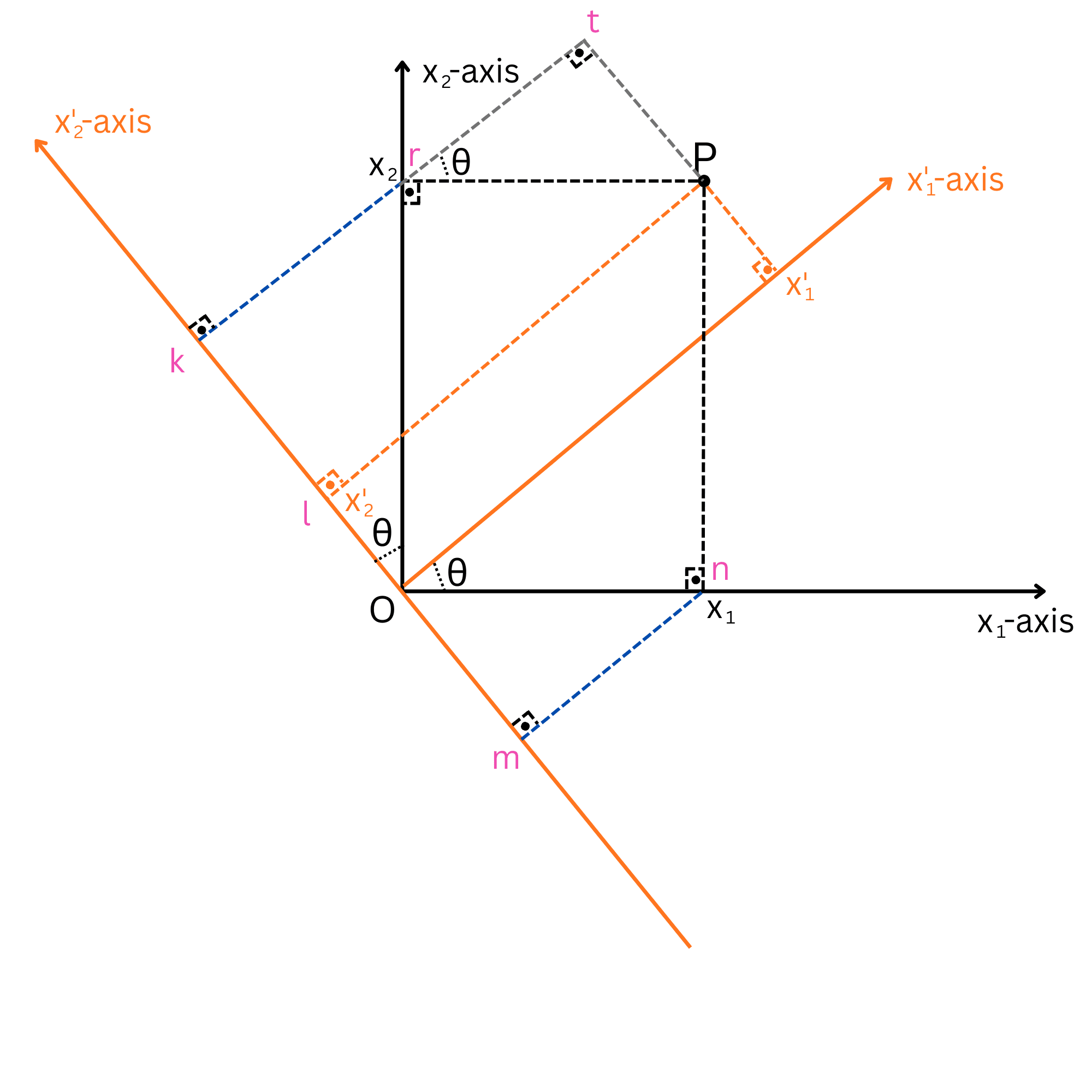
Next, draw a line parallel to $kn‾$ and another line parallel to the $x_1^{\prime }$-axis. Let these two lines intersect at point $t$ (see Figure 3).

Since $\left(kntm\right)$ is a rectangle, the length $nt‾$ is equal to the sum of $kl‾$ and $lm‾$:
$nt‾=kl‾+lm‾$.
Similarly, since $\left(x_{2}OnP\right)$ is a rectangle, we obtain $Pn‾=x_2$. Using the right triangle $$, we have
$nt‾=x_2\sin \theta$.
Therefore, because $nt‾=kl‾+lm‾$, it follows that
$nt‾=kl‾+lm‾=x_2\sin \theta$.
As a result, since $x_1^{\prime }=Ok‾+kl‾+lm‾$, we obtain
$x_1^{\prime }=Ok‾⏟x_1\cos \theta +kl‾+lm‾⏟x_2\sin \theta$.

Finally, we find the new coordinate $x_1^{\prime }$ in terms of $x_1$ and $x_2$ by projecting the $x_1$ and $x_2$ coordinates onto the new $x_1^{\prime }$-axis:
$x_1^{\prime }=x_1\cos \theta +x_2\sin \theta$

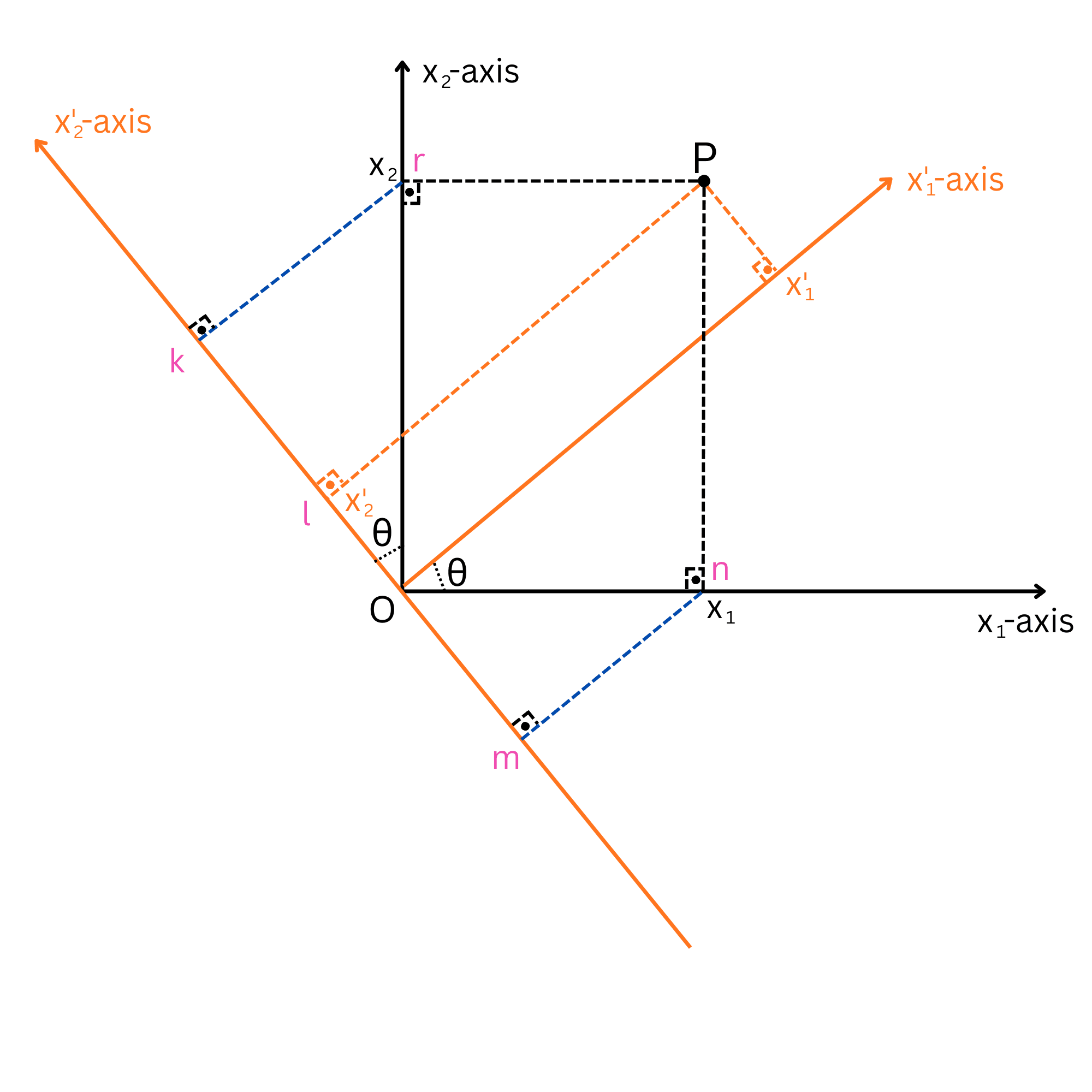
Similarly, assign the labels $k$, $l$, $m$, $n$, and $r$ to the points shown in Figure 4.

Next, determine the projections of $x_1$ and $x_2$ onto the $x_2^{\prime }$-axis. These projections can be written as
${\mathrm{proj}}_{x_2^{\prime }}{x}_1=-Om‾=-x_1\sin \theta$
${\mathrm{proj}}_{x_2^{\prime }}{x}_2=Ok‾=x_2\cos \theta$

These segments represent the components of $x_1$ and $x_2$ along the $x_2^{\prime }$ direction.

Afterward, draw a line through point $r$ parallel to the segment $lP‾$, and draw another line parallel to the $x_2^{\prime }$-axis. Denote the intersection point of these two lines by $t$ (see Figure 5). This construction helps visualize the geometric relationship between the projections and the rotated coordinate axis.

Since triangles $△\left(mnO\right)$ and $△\left(trP\right)$ are similar with similarity ratio 1, i.e. $△\left(mnO\right)\sim △\left(trP\right)$, we obtain $tP‾=Om‾$.
Moreover, since $\left(klPt\right)$ is a rectangle, we have $kl‾=tP‾$, and therefore, using $tP‾=Om‾$, we get $kl‾=Om‾$.
From the geometry of the figure (see Figure 5), it follows that
$lO‾=Ok‾-Om‾$
Finally, since $lO‾=x_2^{\prime }$, $Ok‾=x_2\cos \theta$, and $Om‾=x_1\sin \theta$, substituting into $lO‾=Ok‾-Om‾$ gives $x_2^{\prime }=x_2\cos \theta -x_1\sin \theta$

By combining the two results we obtained, we derive two relations between the old and the new coordinates of point $P$:
$x_1^{\prime }=x_1\cos \theta +x_2\sin \theta x_2^{\prime }=-x_1\sin \theta +x_2\cos \theta$

To generalize this idea, we introduce a useful notation. The direction cosine ${\lambda }_{ij}$ is defined as the cosine of the angle between the new axis $x_i^{\prime }$ and the original axis $x_j$:
${\lambda }_{ij}=\cos (x_i^{\prime },x_j)$
Each ${\lambda }_{ij}$ tells us how much the $j$-th original axis contributes to the $i$-th new axis. Using this notation, the transformation equations become elegant and compact.

In three dimensions, each new coordinate is a linear combination of all three original coordinates, weighted by the appropriate direction cosines:

The inverse transformation — going back from the rotated system to the original — has a very similar form:

It is natural to collect all the direction cosines ${\lambda }_{ij}$ into a square array. This gives us the rotation matrix (also called the transformation matrix):

Each row of this matrix contains the direction cosines for one of the new axes. Once you know $A$, you can transform any point between the two coordinate systems.