Open Physics Letters Logo
AnalysesArticlesCoursesProblemsGreat PhysicistsBooks in Physics History
TRTRENEN
Open Physics Letters

Open Physics Letters provides free access to academic analyses, historical breakthroughs, and educational resources in physics — from high school to postgraduate level.

TR

Academic Content

  • auto_storiesArticles
  • psychologyAnalyses
  • personGreat Physicists
  • menu_bookBooks in Physics History

Education

  • schoolCourses
  • calculateProblem Solutions

Institute

  • About Us
  • Contact
  • Contribute
  • Privacy Policy
  • Terms of Service

© 2026 Open Physics Letters Academic Press. All rights reserved.

TRTR|ENEN
Problem Solutionschevron_rightClassical Mechanicschevron_rightClassical Dynamics of Particles and Systemschevron_rightMatrices, Vectors, and Vector Calculuschevron_rightProblem 1-1
psychology

Problem 1-1

The problem text is not included due to copyright reasons
This page presents only the solutions to the problems; the original problem statement is not shared as it is subject to copyright.
Analytical Solution Steps
1
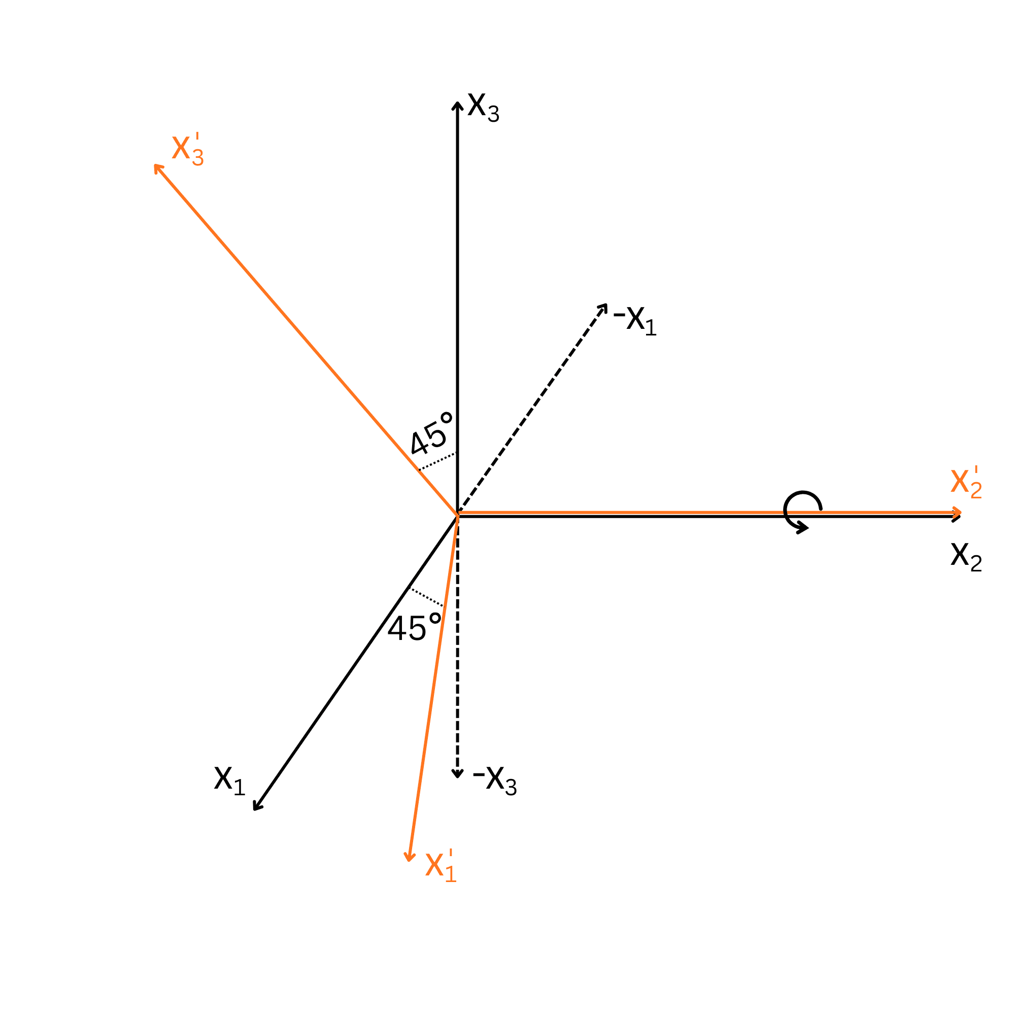
Let us visually illustrate the rotation described in the problem using coordinates.
Let us denote the axes after the rotational motion as x1′x'_1x1′​, x2′x'_2x2′​, and x3′x'_3x3′​. In this case, the configuration of the axes resulting from a 45∘45^{\circ}45∘ rotation about the x2x_2x2​ axis can be represented as shown in Figure-1. As observed in Figure-1, since the rotation is performed about the x2x_2x2​ axis, the x2x_2x2​ axis remains unchanged; therefore, the x2′x'_2x2′​ axis coincides with the original x2x_2x2​ axis in direction. On the other hand, as a result of the rotation, the x1x_1x1​ axis shifts into the region x1>0x_1 > 0x1​>0 and x3<0x_3 < 0x3​<0 within the x1–x3x_1\text{--}x_3x1​–x3​ plane, and is denoted by x1′x'_1x1′​. Similarly, the x3x_3x3​ axis moves into the region x1>0x_1 > 0x1​>0 and x3>0x_3 > 0x3​>0 within the same plane, and is represented by x3′x'_3x3′​.
Step image 1
Figure-1
2
Let us now write the transformation relations.
As seen in Figure~1, the x1′x'_1x1′​ axis lies in the x1–x3x_1\text{--}x_3x1​–x3​ plane within the region x1>0x_1 > 0x1​>0 and x3<0x_3 < 0x3​<0. Therefore, the angle between x1′x'_1x1′​ and the x2x_2x2​ axis is 90∘90^{\circ}90∘, while the angle between x1′x'_1x1′​ and the x1x_1x1​ axis is 45∘45^{\circ}45∘ (see Figure-1). Using these geometric relations, the x1′x'_1x1′​ axis can be expressed in terms of x1x_1x1​, x2x_2x2​, and x3x_3x3​ as x1′=x1cos⁡45∘+x2cos⁡90∘−x3sin⁡45∘x'_1 = x_1 \cos 45^{\circ} + x_2 \cos 90^{\circ} - x_3 \sin 45^{\circ}x1′​=x1​cos45∘+x2​cos90∘−x3​sin45∘ Similarly, since the coordinate system is rotated about the x2x_2x2​ axis, the x2x_2x2​ axis remains unchanged. Consequently, the angle between x2′x'_2x2′​ and the x2x_2x2​ axis is 0∘0^{\circ}0∘, whereas the angles between x2′x'_2x2′​ and the x1x_1x1​ and x3x_3x3​ axes are 90∘90^{\circ}90∘. Accordingly, the x2′x'_2x2′​ axis can be written as x2′=x1cos⁡90∘+x2cos⁡0∘+x3cos⁡90∘x'_2 = x_1 \cos 90^{\circ} + x_2 \cos 0^{\circ} + x_3 \cos 90^{\circ}x2′​=x1​cos90∘+x2​cos0∘+x3​cos90∘ Applying the same reasoning to the x3′x'_3x3′​ axis, it is observed that x3′x'_3x3′​ lies in the x1–x3x_1\text{--}x_3x1​–x3​ plane within the region x1>0x_1 > 0x1​>0 and x3>0x_3 > 0x3​>0. Hence, the angle between x3′x'_3x3′​ and the x2x_2x2​ axis is 90∘90^{\circ}90∘, while the angle between x3′x'_3x3′​ and the x3x_3x3​ axis is 45∘45^{\circ}45∘ (see Figure~1). Using these geometric relations, the x3′x'_3x3′​ axis can be expressed as x3′=x1sin⁡45∘+x2cos⁡90∘+x3cos⁡45∘x'_3 = x_1 \sin 45^{\circ} + x_2 \cos 90^{\circ} + x_3 \cos 45^{\circ}x3′​=x1​sin45∘+x2​cos90∘+x3​cos45∘
3
Let us write the obtained transformation relations together:
x1′=x1cos⁡45∘+x2cos⁡90∘−x3sin⁡45∘x'_1 = x_1 \cos 45^{\circ} + x_2 \cos 90^{\circ} - x_3 \sin 45^{\circ}x1′​=x1​cos45∘+x2​cos90∘−x3​sin45∘ x2′=x1cos⁡90∘+x2cos⁡0∘+x3cos⁡90∘x'_2 = x_1 \cos 90^{\circ} + x_2 \cos 0^{\circ} + x_3 \cos 90^{\circ}x2′​=x1​cos90∘+x2​cos0∘+x3​cos90∘ x3′=x1sin⁡45∘+x2cos⁡90∘+x3cos⁡45∘x'_3 = x_1 \sin 45^{\circ} + x_2 \cos 90^{\circ} + x_3 \cos 45^{\circ}x3′​=x1​sin45∘+x2​cos90∘+x3​cos45∘ Since sin⁡45∘=cos⁡45∘\sin 45^{\circ} = \cos 45^{\circ}sin45∘=cos45∘, these transformation equations can be written in the following simplified form: x1′=x1cos⁡45∘+x2cos⁡90∘−x3cos⁡45∘x'_1 = x_1 \cos 45^{\circ} + x_2 \cos 90^{\circ} - x_3 \cos 45^{\circ}x1′​=x1​cos45∘+x2​cos90∘−x3​cos45∘ x2′=x1cos⁡90∘+x2cos⁡0∘+x3cos⁡90∘x'_2 = x_1 \cos 90^{\circ} + x_2 \cos 0^{\circ} + x_3 \cos 90^{\circ}x2′​=x1​cos90∘+x2​cos0∘+x3​cos90∘ x3′=x1cos⁡45∘+x2cos⁡90∘+x3cos⁡45∘x'_3 = x_1 \cos 45^{\circ} + x_2 \cos 90^{\circ} + x_3 \cos 45^{\circ}x3′​=x1​cos45∘+x2​cos90∘+x3​cos45∘
4
Let us express the transformation equations in matrix form:
[x1′x2′x3′]=[cos⁡45∘cos⁡90∘−cos⁡45∘cos⁡90∘cos⁡0∘cos⁡90∘cos⁡45∘cos⁡90∘cos⁡45∘][x1x2x3]\begin{bmatrix} x'_1 \\ x'_2 \\ x'_3 \end{bmatrix} = \begin{bmatrix} \cos 45^{\circ} & \cos 90^{\circ} & - \cos 45^{\circ} \\ \cos 90^{\circ} & \cos 0^{\circ} & \cos 90^{\circ} \\ \cos 45^{\circ} & \cos 90^{\circ} & \cos 45^{\circ} \end{bmatrix} \begin{bmatrix} x_1 \\ x_2 \\ x_3 \end{bmatrix}​x1′​x2′​x3′​​​=​cos45∘cos90∘cos45∘​cos90∘cos0∘cos90∘​−cos45∘cos90∘cos45∘​​​x1​x2​x3​​​
5
Let us substitute the cosine values.
Using cos⁡45∘=12\cos 45^{\circ} = \dfrac{1}{\sqrt{2}}cos45∘=2​1​ and cos⁡90∘=0\cos 90^{\circ} = 0cos90∘=0 in the matrix equation, we obtain [x1′x2′x3′]=[120−1201012012][x1x2x3]\begin{bmatrix} x'_1 \\ x'_2 \\ x'_3 \end{bmatrix} = \begin{bmatrix} \dfrac{1}{\sqrt{2}} & 0 & - \dfrac{1}{\sqrt{2}} \\ 0 & 1& 0 \\ \dfrac{1}{\sqrt{2}} & 0 & \dfrac{1}{\sqrt{2}} \end{bmatrix} \begin{bmatrix} x_1 \\ x_2 \\ x_3 \end{bmatrix}​x1′​x2′​x3′​​​=​2​1​02​1​​010​−2​1​02​1​​​​x1​x2​x3​​​
6
As a result, the 3×33 \times 33×3 matrix obtained in this expression represents the transformation matrix requested in the problem:
[120−1201012012]\begin{bmatrix} \dfrac{1}{\sqrt{2}} & 0 & - \dfrac{1}{\sqrt{2}} \\ 0 & 1& 0 \\ \dfrac{1}{\sqrt{2}} & 0 & \dfrac{1}{\sqrt{2}} \end{bmatrix}​2​1​02​1​​010​−2​1​02​1​​​
menu_bookGo to Unit
library_books

Source

menu_bookClassical Dynamics of Particles and Systems
subdirectory_arrow_rightMatrices, Vectors, and Vector Calculus

Problems in Unit

1. Introduction
2. Concept of a Scalar
3. Coordinate Transformations
Problem 1
4. Properties of Rotation Matrices
5. Matrix Operations
6. Further Definitions
7. Geometrical Significance of Transformation Matrices
8. Definitions of a Scalar and a Vector in Terms of Transformation Properties
9. Elementary Scalar and Vector Operations
10. Scalar Product of Two Vectors
11. Unit Vectors
12. Vector Product of Two Vectors
13. Differentiation of a Vector with Respect to a Scalar
14. Examples of Derivatives: Velocity and Acceleration
15. Angular Velocity
16. Gradient Operator
17. Integration of Vectors